Evaluation of the Chinese Slumber prediction method
Jorge Stolfi
May 12, 2014
Last edited on 2014-05-12 01:07:16 by stolfilocal
Executive summary
The Chinese Slumber Method (CSM) is not significantly better than the banal predictor, "tomorrow will be like today" (TLT). Over the last 3 months, CSM has been more accurate than TLT ~60% of the time, but on the other ~40% attempts its errors are much larger, so its root-mean-square error is larger than TLT's. However there may be room for improvement.
Goal and premises of the CSM
The Chinese Slumber Method tries to predict the CNY/BTC price at Huobi in the late night hours of the next day (around 03:30 am, China time), from the price and volume at the same hour of the preceding days.
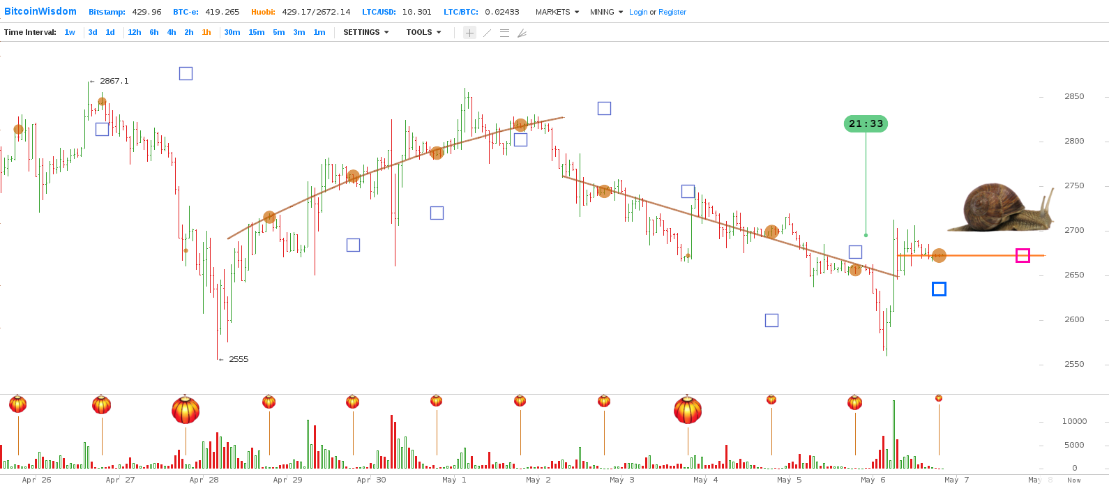
At those [i]slumber times[/i], Huobi's volume is minimal, so it is hoped that the price at those times is more stable and better reflects the underlying fundamental factors -- basically, the expectations of traders and the availability of money and bitcoins in the market. Those numbers are expected to be more reliable for prediction purposes than the price at any other hour, and even better than the daily average price. Here is some visual evidence for that claim:
 [click on image to see a full-size version ]
In this plot, the yellow dots are the [i]slumber points[/i], the prices at the slumber times. Note that the four points Apr/29--May/02 fall on a smooth trend line, while the price swings wildly between them (from about 06:00 am to 01:00 am China time).
The price changes are due in part to gradual changes in the fundamental factors, spanning several days. It is these gradual changes that the CSM aims to detect and extrapoalte. In addition to those gradual changes, the price obviously undergoes sudden [i]trend breaks[/i] caused by discrete events, such as news about bitcoin, government regulations, changes in the trading fees, deadlines, etc.. Needless to say, the CSM cannot predict such discrete events. Finally, the price includes a substantial random (hence unpredictable) component; which the CSM tries to avoid by considering only the prices at slumber times.
The CSM was devised specifically for Huobi, and is not expected to work for other exchanges that have round-the-clock activity, low liquidity, significative interference from arbitrage, or other disturbing factors. However, the USD/BTC price at Bitstamp has usually tracked the CNY/BTC price at Huobi, by an [i]effective currency exchange factor[/i] R that is close, but not equal, to the official CNY/USD exchange rate. Thus a prediction for Bitstamp has been provided by computing the R factor at the last few slumber times, extrapolating it to the next slmber time, and applying it to the Huobi prediction above.
[click on image to see a full-size version ]
In this plot, the yellow dots are the [i]slumber points[/i], the prices at the slumber times. Note that the four points Apr/29--May/02 fall on a smooth trend line, while the price swings wildly between them (from about 06:00 am to 01:00 am China time).
The price changes are due in part to gradual changes in the fundamental factors, spanning several days. It is these gradual changes that the CSM aims to detect and extrapoalte. In addition to those gradual changes, the price obviously undergoes sudden [i]trend breaks[/i] caused by discrete events, such as news about bitcoin, government regulations, changes in the trading fees, deadlines, etc.. Needless to say, the CSM cannot predict such discrete events. Finally, the price includes a substantial random (hence unpredictable) component; which the CSM tries to avoid by considering only the prices at slumber times.
The CSM was devised specifically for Huobi, and is not expected to work for other exchanges that have round-the-clock activity, low liquidity, significative interference from arbitrage, or other disturbing factors. However, the USD/BTC price at Bitstamp has usually tracked the CNY/BTC price at Huobi, by an [i]effective currency exchange factor[/i] R that is close, but not equal, to the official CNY/USD exchange rate. Thus a prediction for Bitstamp has been provided by computing the R factor at the last few slumber times, extrapolating it to the next slmber time, and applying it to the Huobi prediction above.
Reliability weights
When a slumber point falls away from the surrounding trend line(s), it is often the case that Huobi's clients kept trading until late that night. Thus the CSM defines a [i]reliability weight[/i] W for each point, based on the trade volume in between 02:00 and 04:59 am, compared to the total volume for that day. The exact definition of the weight is at the end of this note; for now it suffices to say that W varies from 0 (lots of late night trade) to 1 (no late night trade at all). In the above plot, the area of each lantern is propotional to the relative late night volume, and the area of each yellow dot is proportional to its weight W.
The weight W is used in the CSM in several ways: to evaluate whether a data point is to be trusted when choosing the type of trend line, to specify the point's infuence when fitting trend lines to multiple points, and to guess whether a trend break occurred. For example, the three slumber points of May/03, 05, and 06, which have W near 1, lie almost in a straight line; whereas the point of Mar/04, that lies far from that line, has W near zero.
The following plots shows the slumber points from 2014-01-15 to 2014-05-09:
 [click on image to see a full-size version ]
Note that the points with W near 1 (largest dots) tend to vary gradually, following smooth trends for several says at a time; while points with W near 0 (smallest dots) often lie off the trend of the largest dots.
[click on image to see a full-size version ]
Note that the points with W near 1 (largest dots) tend to vary gradually, following smooth trends for several says at a time; while points with W near 0 (smallest dots) often lie off the trend of the largest dots.
Trend identification
After each slumber point is observed, the CSM considers the last few points and tries to identify which ones are part of the current trend, if any. This part of the method is still partly subjective, although it can be automated by the dynamic programming method. A mathematical formula is then fitted to those points by the weighted least squares method. The next slumber point is then predicted from this formula.
The mathematical formula is restricted to a straight line A + B*(d-d0) or a shifted decaying exponential (SDE) of the form A + B*Q^(d-d0), where (d-d0) is the number of days since the start of the trend, and A, B, and Q are parameters to be determined (with Q between 0 and 1). The decaying exponential is a natural model for quantities in physical systems that gradually tend to some equilibrium value after a sudden transient. The straight line is actually a limiting case of the shifted exponential for Q tending to 1. (Logically, these computations should be carried out in log scale; but, for the short time frame in question, the effect would not be noticeable.)
Points with very low W ([i]bad[/i] points) are largely ignored in the choice of the trend, while points with W close to 1 ([i]good[/i] points) must be considered. Points with intermediate W may or may not be considered, depending on how well they fit the pattern of the nearby good points.
In general, the last two good points are assumed to be on the current trend, unless they are more than 2-3 days in the past or separated by more than 2-3 bad points. If there is a straight line or SDE that also lies close to one or more previous good points, those points are assumed to be part of the trend too.
If these criteria select only two good points, then the trend is taken to be a straight line. If they select three or more good points, the method generally considers the trend to be an SDE. In this case, the ratio Q is determined manually as the ratio (P2-P1)/(P1-P0), where P0, P1 and P2 are the prices at the first, middle, and last selected times. (The middle point may have to be interpolated, e.g. graphically.) In either case, the parameters A and B are determined by weighted least squares, using all the points, good or bad, in that time interval. A straight line may be used instead of an SDE it the fit turns out to be just as good (that is, if Q is close enough to 1).
When the criteria fail to identify two good points to define the trend (usually because there were too many bad points in the preceding days), the method returns a "desperate" prediction that is just the price at the last good point if it is not too remote, or the last slumber point otherwise.
Evaluation
I have compared the CSM to the banal "Tomorrow Like Today" (TLT) method. The data for each day is provided in two files, one for Huobi and one for Bitstamp. The format is described at the top of each file. The relevant columns are the weight W, the actual price PM at the slumber time (the average of low and high price in the one-hour interval 19:00--19:59 UTC = 03:00--03:59 CST), the Chinese Slumber Method prediction PS, and the banal TLT prediction PB. The lines with PS = 0 are days when no CSM prediction was posted, or two CSM predictions were posted for the same day.
The following scatterplots show the errors ES = PS-PM and EB = PB-PM of the CSM and TLT methods, respectively:
[click on image to see a full-size version ]
Conclusions
The Chinese Slumber Method is not a useful predictor in its current form.
Its premises do seem valid: (1) the prices at slumber times seem to follow simple trends over several days, broken by unpredictable discontinuities clearly linked to discrete events; and (2) high relative trading volume around the slumber times is correlated with deviations from the current trend, which often resumes after those "bad" data points.
However, the current trend often can be identified only after three days, or more when there are bad points; and since a trend has rarely lasted unbroken more than four days, it follows that the prediction is more often based on the wrong trend than on the correct one.
Nevertheless, the experiment has inspired an efficient algorithm for fitting a piecewise polynomial function to a set of data points, which is now being implemented and tested.