[Previous chapter] [Next chapter]

Stochastic Programming (SP) basics

---

Stochastic problems can essentially be divided into 2-stage and multi-stage problems. In a 2-stage problem, the initial decisions are taken first. These are then followed by a random event. Next, the recourse decisions, which are based on this random event, are taken. The multi-stage problem, as the name suggests, consists of multiple stages, with a random event occurring between each stage. In this case, decisions are made at each stage. The following sections give a detailed description of these problems:

2-stage stochastic problems

In a 2-stage problem, first, the initial or the first stage decisions (e.g., system design decisions) are made which are followed by random events such as demand, availability, price, or a combination of these. Then the second stage decisions (e.g. operational decisions) are made. This can be viewed pictorially as follows:

Figure 3.1: 2-stage problem

In the standard form, the 2-stage stochastic program is:

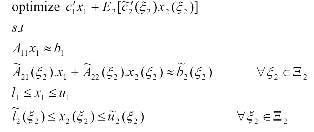
where indicates , , = or combination of these. x₁ and x₂ are the first and the second stage stochastic decision variables respectively. E₂[] is the expectation operator with respect to the random event ₂. ₂ represents the state space (the set of possible outcomes or the values that ₂ can assume) in the recourse stage. There may be separate values for the objective coefficients c˜'₂(₂), right hand side b˜₂(₂), and matrix coefficients Ã₂₁(₂) and Ã₂₂(₂) for each outcome ₂ in ₂, and the recourse decisions x₂(₂) depend on ₂, i.e., there are separate sets of recourse decisions for each outcome ₂ in the second stage.

Multi stage stochastic problems

Multi-stage problems can be viewed pictorially as follows:

Figure 3.2: Multi-stage problem

Formally, the multi-stage stochastic program is defined as follows:

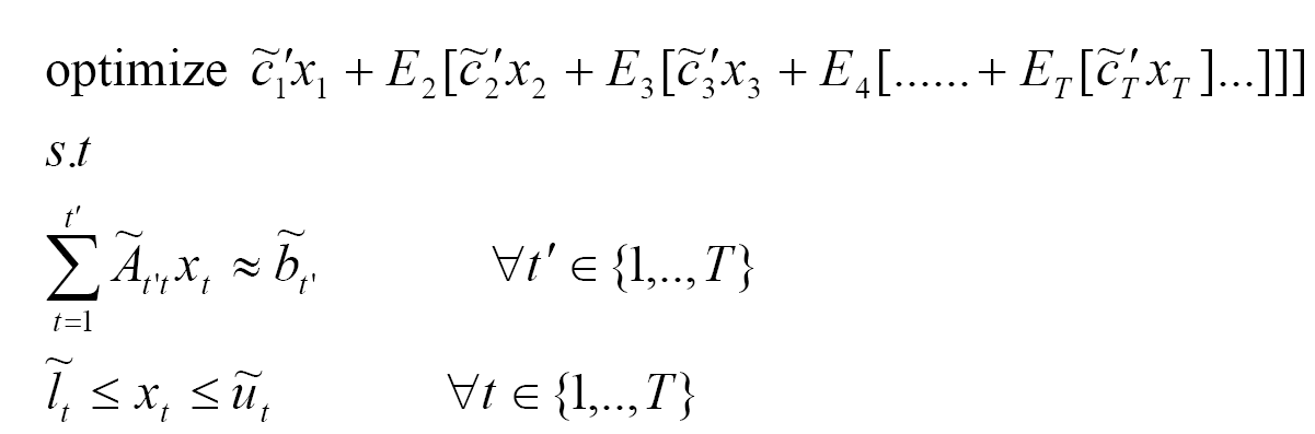
where
`optimize' indicates maximize or minimize
˜ indicates random data variable
indicates , , = or a combination of these

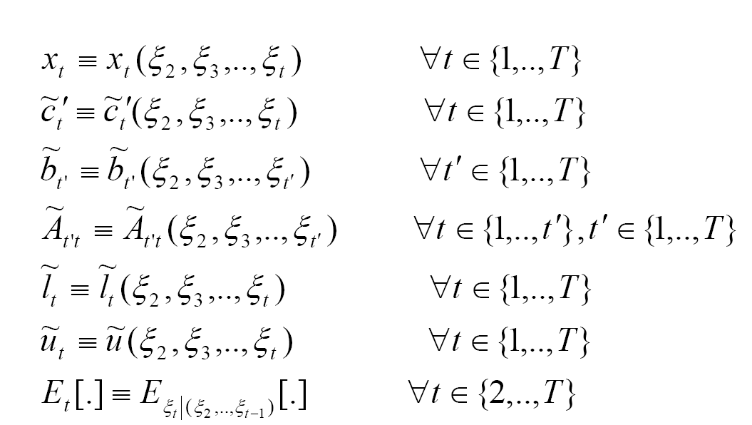
Each of the above entities depends on the sequence of events (₂,₃,...).—Note that c₁, A₁₁, b₁, l₁, and u₁ are not random.—

Scenario generation

_t being a random variable, takes different values with different probabilities. If each of the _t's can be discretized, the realized values of _t give rise to what is called a scenario tree. An example of a scenario tree with T (number of stages) =3 and S (number of scenarios) =4 is shown in Figure 3-stage scenario tree.

Figure 3.3: 3-stage scenario tree

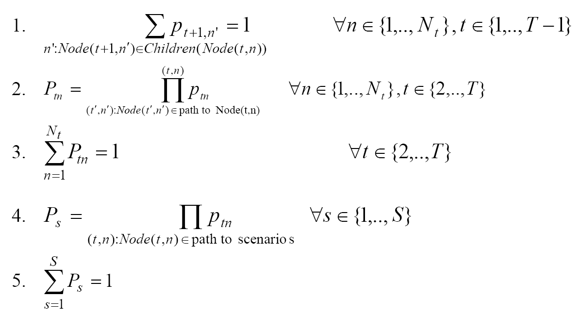
In the t^th stage there are N_t nodes. For each stage t in 2 to T, each _t has N_t outcomes (_t1 w.p. p_t,1,_t2 w.p. p_t,2,..._tNt w.p. p_t,Nt), where p_tn is the conditional probability of visiting the n^th node in the t^th stage from its parent node in the t-1^th stage. The realizations of ₂, ₃,...,_T correspond to scenarios (paths in the tree). For each stage t and each node n in that stage, the node has an unconditional probability P_tn of being visited, which is equal to the product of conditional probabilities along the path to that node. Similarly, each scenario s has a scenario probability P_s that is equal to the product of conditional probabilities along the path to that scenario. The following observations can be made about the scenario tree:

1. 

Underlying deterministic model

If we ignored the randomness of the data momentarily, then an underlying deterministic model can be written as follows:

Expanding the underlying deterministic model

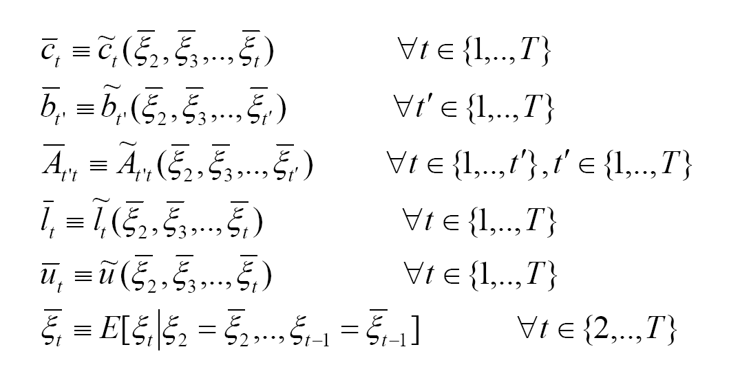
Given the dependency of the coefficients (c˜_t,Ã_tt',b˜_t,l˜_t,u˜_t) of a stochastic program on the random events (_t), it can automatically be expanded into an extensive form (deterministic equivalent problem) by introducing new variables and constraints. There are basically two ways of creating new variables and constraints: node based and scenario based.

Node based

Given a scenario tree, the underlying deterministic model can be expanded into an extensive mathematical program based on the nodes. The basic idea is to add a subscript of a node number to each of the stochastic decision variables (x_t becomes x_t,n for n=1,...,N_t). Then the resulting extensive deterministic model would be:

In this model c_tn,A_tt'n,b_tn,l_tn,u_tn are the resolved values of c˜_t,Ã_tt',b˜_t,l˜_t,u˜_t at the node(t,n). Based on above formulation, the matrix structure of the problem shown in Figure 3-stage scenario tree would look as follows:

Figure 3.4: Node based matrix

Scenario based

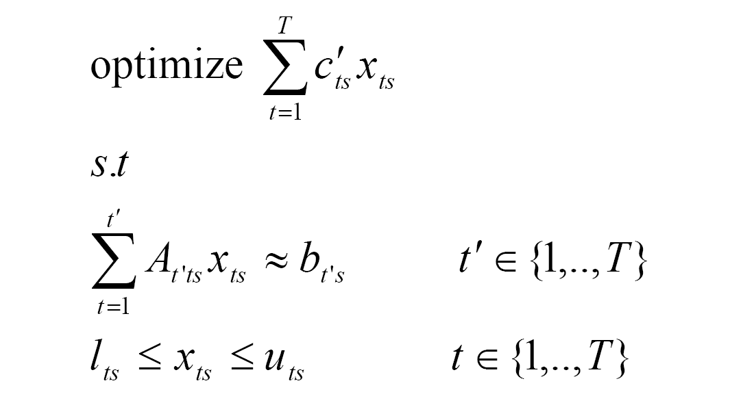
A stochastic model can also be expanded based on the scenarios. Here each variable is also subscripted by scenarios (x_t x_t,s for s=1,...,S). The expanded mathematical program would look as follows:

Here c_ts,A_tt's,b_ts,l_ts,u_ts are realizations of c˜_t,Ã_tt',b˜_t,l˜_t,u˜_t respectively in scenario s.

Non-anticipative constraints (NAC)

Consider the node(2,2) in Figure 3-stage scenario tree. When the model is parsed according to scenarios, although we have two separate variables x₂₂ and x₂₃ corresponding to scenarios 2 and 3 at this node, both of them should assume same value since they cannot depend on the future events (x_t x_t(_s,...,_t)). Therefore, the following set of non-anticipative constraints also needs to be included in the above formulation:
x_ts = x_ts' n {1,...,N_t}, t {1,...,T-1}, s s' _tn, where _tn is the set of scenarios passing through the node(t,n). Hence, the matrix structure for the problem shown in Figure 3-stage scenario tree would look as follows.

Figure 3.5: Scenario based matrix

Solution measures

Recourse problem (R.)

The standard stochastic problem discussed in Section Multi stage stochastic problems is also referred to as the recourse problem.

Expected Value problem

If the _t's are replaced by their expected values in the recourse problem, then such a problem is called an expected value (EV) problem.

where,

Expected Value problem with recourse

Let x^- = (x^-₁,x^-₂,...x^-_T) be the optimal solution to the above problem, then for each stage an expected recourse problem can be defined as follows.

Here, the first t stage variables are fixed at their optimal values obtained in the EV problem. The following observations can be made:

1. z_EV is not worse than z_R (i.e., if maximizing, z_EV z_R).
2. If

   t

   t''=1

   Ã_t't''x^-_t' b˜_t', l˜_t' x^-_t' u˜_t' t'{1,...,t} and EVr^t is feasible then, z_R is not worse than z_EVr(t).
3. If 2. is true then the value of stochastic solution: VSS(t) is the absolute value of the difference between z_R and z_EVr(t), else it is +.

Perfect Information problem

Here, the problem for each scenario is solved independently.

Let x^*_s = (x^*_1s,x^*_2s,...,x^*_Ts) be the optimal solution to the above problem,
x^* =

S

s=1

P_sx^*_s = (x^*₁,x^*₂,...,x^*_T) be the aggregated solution, and z_PI =

S

s=1

P_sz_PI(s) be the aggregated objective value.

Perfect information problem with recourse

The following observations can be made:

1. Z_PI is not worse than Z_RP.
2. If

   t

   t''=1

   Ã_t't''x^*_t' b˜_t', l˜_t' x^*_t' u˜_t' t'{1,...,t} and PIr^t is feasible then, Z_PI is not worse than Z_PIr(t).
3. If 2. is true then the expected value of perfect information: EVPI is the absolute value of the difference between Z_R and Z_PI, else it is +.

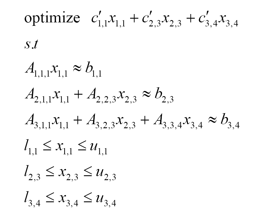
Focus on an instance of the problem

Instead of looking at the fully expanded problem at once, one could also look at the instance of the underlying problem in a particular scenario or at a node in a scenario tree. The corresponding

model in a scenario s

model at a node(t,n) in the scenario tree

e.g. in Figure 3-stage scenario tree the model focused at node(3,4) will be:

[Next] [Index]

---

If you have any comments or suggestions about these pages, please send mail to docs@dashoptimization.com.