Building stochastic models
In this chapter we look in detail at how users can build stochastic models in Xpress-SP using the functionalities available in the mmsp module. The steps and issues related to scenario generation, model formulation, and solution analysis are addressed here. Although the framework for building stochastic models is flexible, users are advised to follow the model-building procedures in a sequential fashion as shown below.
Setting stages
Stages are set using the function spsetstages(Stages: set); e.g.,
 declarations
  T=4
  Stages=1..T
 end-declarations
 spsetstages(Stages)
The set Stages can be of type integer or string, or it can be a range.
SPrands and SPrandexps
Each sprand corresponds
to a stochastic event (![]() t), and hence its stage
and possible values must be set by the user. sprandexps on the
other hand are expressions built using sprand, and therefore their
stages and values are automatically defined.
t), and hence its stage
and possible values must be set by the user. sprandexps on the
other hand are expressions built using sprand, and therefore their
stages and values are automatically defined.
Declaring and associating sprand with stages
Random variables are declared as sprand in mmsp.
 declarations
  demand, price :array(2..T) of sprand
 end-declarations
It is recommended that at the time of declaration of arrays of sprand, all the sets used for indexing such arrays be constant or finalized (i.e. elements of sets are known and sizes of sets are fixed). At the time of declaration, sprand are automatically `created', however if one or more of the sets used for indexing an array of sprand are dynamic then by default such an array is dynamic in nature. In this case, users will have to explicitly create all the sprand using the create procedure (e.g., T:=4; forall(t in 2..T) create(demand(t)).
Users can set the stage of sprand using the function spsetstage(srnd: sprand).
One or more sprand in each stage may correspond to the ![]() t for that stage; e.g.,
t for that stage; e.g.,
 forall(t in 2..T)  spsetstage(demand(t),t)
 forall(t in 2..T)  spsetstage(price(t),t)
In the above example, the pair (demandt, pricet)
corresponds to the random event ![]() t.
Note that users may not have to set the stages of all sprand
if the parameter xsp_implict_stage is set to true
(see Section Setting SP parameters). Also note that one could dissociate an sprand
from a stage by setting its stage to XSP_STAGE_ZERO.
t.
Note that users may not have to set the stages of all sprand
if the parameter xsp_implict_stage is set to true
(see Section Setting SP parameters). Also note that one could dissociate an sprand
from a stage by setting its stage to XSP_STAGE_ZERO.
Operators
The operators: +, -, *, /, and ^ can be used with types real, sprand, and sprandexp to create new spradexp, e.g.,
 declarations
  tot_demand: sprandexp
 end-declarations
 tot_demand:=sum(t in 2..T) demand(t)
Relational conditions
Relational conditions, which themselves are of type sprandexp, can be created using the relational operators: <=, >=, and =, together with real, sprand, and sprandexp.
Logical conditions
Logical conditions, which in turn are of type sprandexp themselves, can be created using relational conditions together with `and', `or', `not' or a combination of these, e.g.,
declarations
  if_demand_demand: sprandexp
 end-declarations
 if_pos_demand:= (demand(2)+demand(3))>=demand(1) or
                  demand(1)>=0
Functions
The general format of all the functions involving sprand and sprandexp is: f(args):sre where f is the name of the function, args are the arguments of this functions, and sre is a sprandexp. This is further described in the following section.
One argument
f: abs, ceil, floor, round, ln, exp
arg1: sprand or sprandexp
Two arguments
f: maximum, minimum
arg1, arg2: real, sprand, or sprandexp
Three arguments
f: spif
arg1: sprandexp (must be a logical or relational condition)
arg2, arg3: real, sprand, or sprandexp (arg2, arg3 correspond to true and false values of the condition)
e.g.,
if sr1, sr2, and sr3 are sprand
then following is a valid usage of spif:
sre:=spif(sr1<=3 and sr1>=sr2^sr3, 1, maximum(sr2,ceil(sr1)))
Here whenever arg1 evaluates to true, sre
is assigned arg2 otherwise it is assigned arg3.
Scenario tree
Generation
The first step in building a stochastic model is the creation of the scenario tree (see e.g. Section Scenario generation).
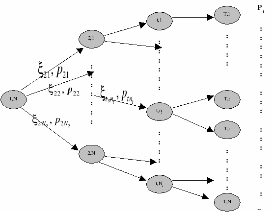
Figure 5.1: Multi-stage scenario tree
where,
T = Number of stages
S = Number of Scenarios
Nt = Number of nodes in stage t (N1=1, NT=S)
Ps = Probability
of scenario s, such that ![]() Ss=1 Ps = 1
Ss=1 Ps = 1
![]() t,nt = Assumed
value of random variable
t,nt = Assumed
value of random variable ![]() t
at node (t,nt)
t
at node (t,nt)
Pt,nt = Conditional probability of occurrence of event ![]() t,nt (at
node (t,nt))
t,nt (at
node (t,nt))
Creation of a scenario tree involves setting of its stages followed by declaration and association of each sprand with a stage.
Exhaustive tree
All independently distributed sprand
If all the random variables in the model are independent, then one can first specify their discretized distribution and generate the tree as follows:
- Assume T=4
- Distribution of demand2 is {5 w.p 0.5, 10 w.p 0.5} in the second stage
- Distribution of demand3 is {7 w.p 0.2, 12 w.p 0.6, 13 w.p 0.2} in the third stage
- Distribution of demand4 is {12 w.p 0.6, 14 w.p 0.4} in the fourth stage
 declarations
  nElem=3
  Elems = 1..nElem
  demand:array(2..T) of sprand
  value,probability:array(2..T,Elems) of real
  val,prob:array(Elems) of real
 end-declarations

 value:=[5,10,0,
         7,12,13,
         12,14,0]
 probability:=[.5,.5,0,
               .2,.6,.2,
               .6,.4,0]

 forall(t in 2..T) do
  forall(e in Elems) prob(e):=0
  forall(e in Elems) prob(e):=probability(t,e)
  forall(e in Elems) val(e):=value(t,e)
  spsetdist(demand(t),val,prob)
 end-do
 spgenexhtree
This will create a tree with 2 branches from first stage nodes, 3 branches from second stage nodes, and 2 branches from third stage nodes, implying a total of 2 · 3 · 2 = 12 scenarios.
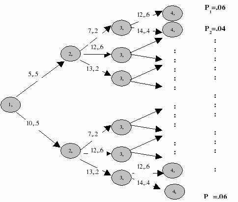
Figure 5.2: Exhaustive scenario tree
Note that in the exhaustive generation, the size of the scenario tree increases rapidly with an increase in the number of sprand. If in the above-mentioned example, we add another random variable pricet, with price2, price3, and price4 assuming 3, 2, and 2 discrete values in the second, third, and fourth stage respectively, then the number of scenarios would be (2 · 3) · (3 · 2) · (2 · 2) = 144.
Some jointly distributed sprand
One can also create a scenario tree with some or all sprand jointly distributed. The following example demonstrates how to build a 3-stage scenario tree, with three sprand namely sr1, sr2 and sr3, where sr1 and sr2 belong to the second stage and sr3 belongs to the third stage. It is assumed that sr1 and sr3 are jointly distributed, whereas sr2 is independently distributed.
 declarations
  T=3
  Stage=1..T
  sr1,sr2,sr3: sprand
 end-declarations

 ! set stages
 spsetstages(Stage)
 spsetstage(sr1,2)
 spsetstage(sr2,2)
 spsetstage(sr3,3)

 ! set independent distribution of sr2 = {10 w.p .2, 20 w.p .8}
 declarations
  ind_val,ind_prob:array(1..2) of real
 end-declarations

 ind_val:=[10,20]
 ind_prob:=[.2,.8]
 spsetdist(sr2,ind_val,ind_prob)

 ! set joint distribution of sr1 and sr3 {(25,45) w.p .3, (35,55)
 w.p .7}
 declarations
  joint_val:array(1..2,1..2) of real
  joint_prob:array(1..2) of real
  SetSrnd:set of sprand
 end-declarations

 joint_val:=[25,35, 45,55]
 joint_prob:=[.3,.7]
 SetSrnd:={sr1,sr3}
 spsetdist(SetSrnd,joint_val,joint_prob)

 ! generate exhaustive tre
 spgenexhtree
The following exhaustive tree is created:
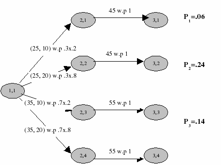
Figure 5.3: Exhaustive scenario tree with some jointly distributed random variables
Stage symmetric
Creating trees
Users may also want to create symmetric trees, e.g., a tree with three branches from each node in each stage. This can be done using the function
spcreatetree(3)
Users must specify the realized values and the conditional or the scenario probabilities afterwards. Similarly, a tree with two branches from the first stage node, 3 branches from each node in the second stage, and 2 branches from each node in the third stage, can be generated as follows:
 declarations
  branches:array(2..T) of integer
 end-declarations
 branches:=[2,3,2]
 spcreatetree(branches)
Specifying values of sprand and conditional probabilities
Once a tree is created explicitly, the default value of all sprand in the scenario tree is zero. mmsp provides functions for setting the assumed value of sprand in the scenario tree based on the tree's structure. If the tree is symmetric with respect to stage (or is symmetric across all the stages), then it can be accomplished as follows:
! Assume branches:=[2,3,2] is already set
 declarations
  MaxBranch=3
  Branches=1..MaxBranch
  value:array(2..T,Branches) of real
  Val:array(Branches) of real
  probability:array(2..T,Branches) of real
  prob:array(Branches) of real
 end-declarations

 value:=[5,10,0,
         7,12,13,
        12,14,0]
 forall(t in 2..T) do
  forall(b in Branches) Val(b):=value(t,b)
  spsetrand(demand(t),Val)
 end-do
 probability:=[.5,.5,0,
               .2,.6,.2,
               .6,.4,0]
 forall(t in 2..T) do
  forall(b in Branches) prob(b):=probability(t,b)
  spsetcondprob(t,prob)
 end-do
This will generate a scenario tree as shown in Figure Exhaustive scenario tree.
Explicit tree
Users may also create a tree (usually asymmetrical) using the following functionalities in mmsp:
Creating a tree
Assume T=3, and user wants to create the following tree
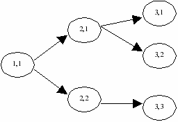
Figure 5.4: Explicit scenario tree - node numbers
- In one shot:
This can be achieved as follows:declarations T=3 ! Number of stages S=3 ! Number of scenarios NodeNum:array(1..S,1..T) of integer end-declarations NodeNum:=[1,1,1, 1,1,2, 1,2,3] spcreatetree(NodeNum)Here, the array NodeNum is created by sequentially entering the node number across the stages for each scenario; e.g., in the second scenario, the node numbers corresponding to the first, second and third stage are 1, 1 and 2 respectively, hence the second row of NodeNum in the above example is [1,1,2]. - Node by node:
Alternatively, the tree can be created as follows:spaddchildren(1,1,2) spaddchildren(2,1,2) spaddchildren(2,2,1)
Here, the function spaddchildren(t,n,b) adds b children nodes at node(t,n).
Creating a tree with trap stages
A tree with a trap stage consists of at least one path that does not necessarily end at the last stage. An example of such a tree is shown in the following figure:
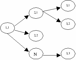
Figure 5.5: Explicit scenario tree - node numbers
Such a tree can also be built using the function spcreatetree(NodeNum) as shown earlier where,
 S=4;
 NodeNum:=[1,1,1,
           1,1,2,
           1,2,0,
           1,3,3];
Note that the stochastic problem associated with such a tree cannot be scenario based, since all scenarios don't exist, therefore xsp_scen_based must be set to false.
Setting realized sprand and probabilities
An sprand can be set using the function spsetrandatnode, e.g.,
 declarations
  N:array(1..T) of integer     ! Total number of nodes in each stage
  value:array(2..T,1..S) of real
  probability: array(2..T,1..S) of real
 end-declarations
 N:=[1,2,3]
 value:=[5,10,0,
         7,12,13]
 forall(t in 2..T,n in 1..N(t)) spsetrandatnode (demand(t),n,value(t,n))
 probability:=[.5,.5,0,
               .2,.8,1]
 forall(t in 2..T,n in 1..N(t)) spsetprobcondatnode (t,n, probability(t,n))
The scenario tree thus created would look as follows:
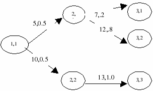
Figure 5.6: Explicit scenario tree - values and probabilities
For the scenario-based problems, users may set the scenario probabilities explicitly using the function spsetprobscen(scen_num: integer, prob: real).
Manipulation
Xpress-SP supports a few scenario manipulation routines such as aggregation and deletion of scenarios. Scenario manipulation can also be done interactively in Xpress-IVE (see Section Analyzing in IVE).
Aggregating all scenarios emerging from a common ancestral node
All the scenarios emerging from an ancestral node in a scenario tree can be aggregated to create one aggregated scenario. Consider following scenario tree:
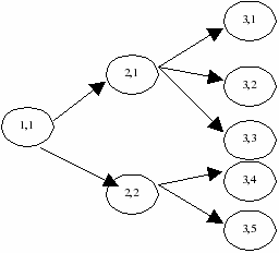
Figure 5.7: Original scenario tree
Here, scenarios 1 to 3 can be aggregated as follows:
spaggregate(1..3)
Note that the new scenario tree is renumbered as follows:
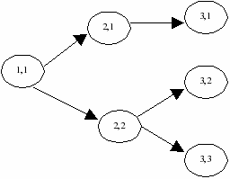
Figure 5.8: Aggregated scenario tree - scenarios 1 to 3
Hence, in order to aggregate scenarios 1 to 3 and scenarios 4 to 5 shown in Figure Original tree separately, the function call should be made in the following order:
 spaggregate(4..5)
 spaggregate(1..3)
This will result in the following tree:
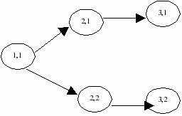
Figure 5.9: Aggregated scenario tree - scenarios 1 to 3 and 4 to 5
Similarly, scenarios 1 to 5 can be aggregated to create a one-scenario scenario tree.
Aggregated probabilities
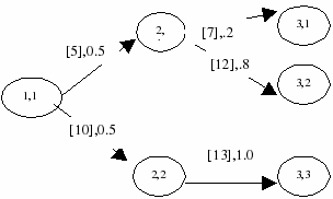
Figure 5.10: Original tree
If scenarios 1 to 2 were aggregated in the above shown tree, the new tree with aggregated values and probabilities would look as follows:
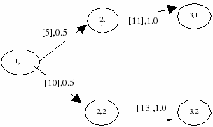
Figure 5.11: Aggregated values
Here, 7 · .2 + 12 · .8 = 11 with probability 1.0. The probability of the aggregated scenarios is the sum of probabilities of the scenarios aggregated.
Aggregating selected scenarios emerging from a common ancestral node
One may also aggregate a set of scenarios (not necessarily contiguous), if none of the nodes after the common ancestral node of the selected scenarios in the path pertaining to the selected scenarios have any siblings. This is illustrated in the following example:
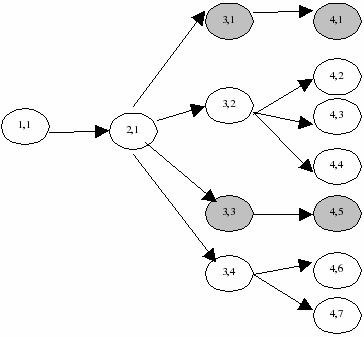
Figure 5.12: 4-stage scenario tree
In the scenario tree shown above, scenarios 1 and 5 can be aggregated since the node(3,1), node(3,3), node(4,1), and node(4,5) lying after the common ancestral node(2,1) do not have any siblings. The corresponding function call in mmsp would be spaggregate({1,5}).
On aggregation, the nodes corresponding to the selected scenarios are deleted. The new aggregated branch corresponding to the aggregated scenario is appended as the last child of the common ancestral node, and the tree node numbers are updated suitably. The aggregated scenario tree in the above example would look as follows:
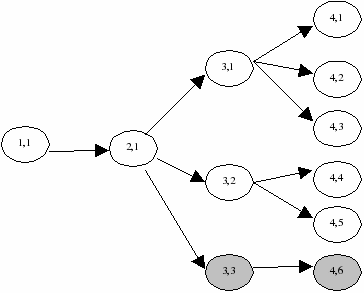
Figure 5.13: Aggregated tree
Deletion in scenario based problems
Users can delete a scenario using the function spdelscen(s:integer). In this case, the probabilities of the remaining scenarios are re-normalized (i.e., each remaining scenario's probability is divided by one minus probability of deleted scenario). Similarly a set of scenarios can be deleted using the function spdelscen(delSet :set of integer). Again, the probabilities are re-normalized (i.e., each remaining scenario's probability is divided by one minus the sum of probability of deleted scenarios), and based on the updated scenario probabilities, the conditional probabilities are re-normalized. The sprand remain unchanged, whereas the node numbers are updated suitably. This is illustrated pictorially in the following example.
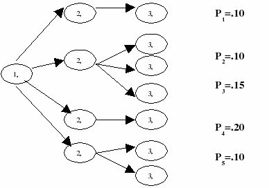
Figure 5.14: 3-stage scenario tree - scenario based
If scenarios 3 and 5 are deleted using the function spdelscen({3,5}), the resulting scenario tree would look as follows:
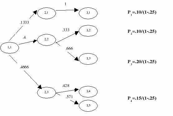
Figure 5.15: Pruned 3-stage tree - scenario based
Deletion in node based problems
Deletion in node-based problems is similar to the one in scenario-based problems, with the exception that the re-normalization of the probabilities is done based on the conditional probabilities of the nodes associated with the deleted scenarios. The following example demonstrates deletion of set of scenarios in a node based problem:
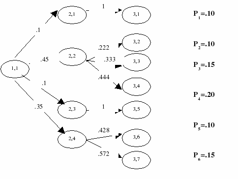
Figure 5.16: 3-stage scenario tree - node based
If scenarios 3 and 5 are deleted using spdelscen({3,5}), then the resulting scenario tree looks as follows:
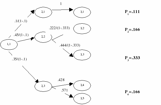
Figure 5.17: Pruned 3-stage tree - node based
Traversing
Users may use several scenario tree related functions such as:
- spgetscencount: to get total number of scenarios (S)
- spgetnodecount(t): to get total number of nodes at stage t (Nt)
- spgetparent(t,n): to get the node number of the parent of node(t,n)
- spgetchildrencount(t,n): to get total number of children nodes of node(t,n)
- spgetchild(t,n,b): to get node number of bth child of node(t,n)
- spgetprobscen(s): to get unconditional probability of sth scenario (Ps)
- spgetprobcond(t,n): to get conditional probability of node(t,n) (ptn)
- spgetprobuncond(t,n): to get unconditional probability of node(t,n) (Ptn)
Evaluating
One can evaluate the realized value of sprands and sprandexps in the scenario tree using the function speval(sptype,scen):real or speval(sptype,stage,node):real e.g., if sr1 and sr2 are of type sprand, and sre is an sprandexp, then the value of sre:=sr1+sr2 at the fourth node in the third stage can be evaluated by calling the function speval(sre,3,4). Calling speval(sre) would return the expected value of sre.
Debugging
One can print the scenario tree loaded in Xpress-SP by calling the function spprinttree.
Formulation
Formulating a stochastic problem in the Xpress-SP syntax involves declarations of spvar and splinctr. The model formulation is discussed below.
Stochastic variables and constraints
Each stochastic variable must be associated with a stage. The stage of a constraint is automatically defined by the stages of the variables and other stochastic entities used to build the constraint.
Declaring and associating spvar with stages
The spvar are declared as follows:
 declarations
  x:array(1..T) of spvar
 end-declarations
It is recommended that at the time of declaration of arrays of spvar, all the sets used for indexing such arrays are `finalized' (i.e. elements of sets are known and sizes of sets are fixed). At the time of declaration, spvar are automatically `created', however if one or more of the sets used for indexing an array of spvars are not `finalized' (e.g. in the above example, if the value of T is not known at the time of declaration), then by default such an array is `dynamic' in nature. In this case, users will have to explicitly `create' all the spvar using the procedure create (e.g., T:=4; forall(t in 1..T) create(x(t))).
Spvars may be associated with a stage (unless xsp_implict_stage is set to true (see Section Setting SP parameters)) e.g.
forall(t in 1..T) spsetstage(x(t),t)
One could also disassociate a spvar from a stage by setting its stage to XSP_STAGE_ZERO.
Setting types and bounds
The type of decision variables can be set using the is_integer, is_binary, and is_free attributes. The bounds can be set by using unnamed unary constraints, e.g., if x is of type spvar and srn is of type sprandexp, then the constraint x<=srn sets the upper-bound of x. Of course, the bounds can be real, sprand or sprandexp.
Writing the objective function and constraints
The objective function and constraints (type splinctr) may be declared as follows:
 declarations
  Obj, Ctr:splinctr
 end-declarations
The following points must be kept in mind while a writing model in Xpress-SP:
- The objective function must be unconstrained (i.e., without a
 ,
,  , or =).
- An splinctr has an implied stage, which is the maximum of the highest stage of sprand and the highest stage of spvar in that splinctr.
- Users may set the type of a splinctr as special ordered set (is_sos1, is_sos2) or as a global constraint (spsettype(Ctr, XSP_GLOBAL)) that chains terms across different realizations in a scenario tree weighted by probabilities of realizations. Special ordered set type constraints cannot contain `fixed' variables (see Section Writing the objective function and constraints), and global constraints cannot occur in expected value (see Section Expected Value problem) or focused (see Section Focus on an instance of the problem) problems.
- In a node based problem, for each spvar in the objective function, the stage of the sprand in its coefficient must not be greater than the stage of the spvar itself (see Section Multi stage stochastic problems).
Manipulation
spvar may be fixed at a certain value using the function spfix(x: spvar, val: real). spunfix can be used on spvar to unfix them. Similarly, splinctr may be hidden or unhidden using the function spsethidden(c: splinctr, cond: boolean). If the second is true, then the constraint is hidden, else it is unhidden. Note that if all the variables of a constraint are fixed, then the constraint is automatically hidden. These functionalities are particularly useful if the user wants to fix some variables e.g., the entire first stage variables at a pre-determined value and solve the problem in the recoursed stochastic framework (see Section Solution measures).
Stochastic problem
The stochastic problem is automatically generated when optimization routine (maximize or minimize) is called. The type of the matrix generated depends on whether the problem is node based or scenario based. Additionally, related problems may also be generated by passing suitable options to the optimization routine.
Setting Xpress optimizer control variables
Users may set the optimizer control parameters using the function setparam e.g., setparam('xprs_presolve',0) will turn the presolve off. All the controls related to the optimizer are listed in the mmsp module.
Optimizing
The problem can be optimized by calling the procedures maximize(Obj: splinctr) or minimize(Obj: splinctr). At this point, the validity of the scenario tree is checked. If no tree exists then an exhaustive tree is attempted to be built (by calling the function spgenexh internally). The problem is then internally expanded and sent to the optimizer. The optimizer control parameters for this problem are also set.
Instance of problem in a scenario
Instead of optimizing the fully expanded problem, once could optimize an instance of a problem in a particular scenario s (see Section Focus on an instance of the problem) by calling maximize(Obj: splinctr, s: integer) or maximize(Obj: splinctr, s: integer). Note that the parameter xsp_scen_based should be set to true.
Instance of problem at a node in the scenario tree
Similarly one could optimize an instance of a problem at a particular node(t,n) (see Section Focus on an instance of the problem) in a scenario tree by calling maximize(Obj: splinctr, t: integer, n: integer) or maximize(Obj: splinctr, t: integer, n: integer). Note that the parameter xsp_scen_based should be set to false.
Options
Users may also pass an option string to indicate the algorithm and type of problem to be solved by calling the function maximize(Obj: splinctr, option: string) or minimize(Obj: splinctr, option: string). The options and their meanings are listed below:
- XSP_OPT_LP_ONLY: solve LP only
- XSP_PRIMAL: use primal simplex
- XSP_DUAL: use dual simplex
- XSP_BARRIER: use barrier
- XSP_REC: solve recourse problem
- XSP_EV: solve expected value problem (see Section Expected Value problem)
- XSP_PI: solve perfect information problem (see Section Perfect Information problem)
- XSP_REC+XSP_EV: solve recoursed expected value problem by fixing first stage variables and hiding first stage constraints (see Section Expected Value problem with recourse).
- XSP_REC+XSP_PI: solve recoursed perfect information problem by fixing first stage variables and hiding the first stage constraints (see Section Perfect information problem with recourse).
As an example, if the user wants to maximize `Profit' — an splinctr — by solving only the LP relaxation of a 4-stage mixed integer problem in a recoursed expected value framework by fixing first stage variables at their expected values and hiding the first stage constraints, using Xpress' barrier routine, the corresponding function call would be:
maximize(Profit, XSP_OPT_LP_ONLY+XSP_BARRIER+XSP_EV+XSP_REC)
Exporting problems
Using the optimization routines spexportprob, maximize or minimize and the constants defined in Xpress-SP one could also export problems. The spexportprob procedure is overloaded as follows:
- spexportprob(dir,objfn,filetype)
- spexportprob(dir,objfn,filetype,filename)
where argument,
- dir can be XSP_MAX or XSP_MIN
- objfn is the objective function of type splinctr
- filetype can be XSP_X_LP, or XSP_X_SP, or XSP_X_SMPS, or XSP_X_SMPS_FREE
- filename is the name of the file in which the exported problem will be stored.
SP file
For the purpose of debugging the underlying SP model, one could export the problem .sp file. For instance, spexportprob(XSP_MIN, Obj, XSP_X_SP, 'myfile') will export the problem in the file myfileProb.sp, whereas minimize(Obj, XSP_X_SP) will both export the stochastic problem in the file ObjProb.sp as well as minimize the problem.
SMPS files
The time, core, and scenario files pertaining to stochastic problem can be exported .e.g., in the free format by calling exportprob(XSP_MAX, obj, XSP_X_SMPS_FREE). This will create the files objSMSP.tim, objSMSP.sto, and objSMPS.cor. Alternatively user may create these files and optimize the problem by calling maximize(obj, XSP_X_SMSP_FREE). Note that if the constant XSP_X_SMSP is used then files are exported in the fixed format.
LP problem
The problem currently loaded in the optimizer can be exported in an lp file by calling spexportprob(XSP_MAX, obj, XSP_X_LP) or maximize(obj, XSP_X_LP).
Getting attributes of a problem from the optimizer
If problem is solved using Xpress optimizer, users may get the status of the problem after optimization by obtaining various integer, real, and string attributes using the function getparam. It is advised that the user checks the optimization status, e.g., xprs_lpstatus and/or xprs_mipstatus, before getting the values of the objective function and other related solutions, comparing the values of these attributes with the constants — XSP_LP_OPTIMAL, XSP_LP_INFEAS, XSP_LP_CUTOFF, XSP_LP_UNFINISHED, XSP_LP_UNBOUNDED, XSP_LP_CUTOFF_IN_DUAL, XSP_MIP_NOT_LOADED, XSP_MIP_LP_NOT_OPTIMAL, XSP_MIP_LP_OPTIMAL, XSP_MIP_NO_SOL_FOUND, XSP_MIP_SOLUTION, XSP_MIP_INFEAS, or XSP_MIP_OPTIMAL.
Getting solution
If the problem is feasible then users can obtain the solution value and reduced cost of spvar, and the activity or slack value of splinctr in a scenario or at a node in the scenario tree. The values of the first stage entities can be found using the following functions:
 getsol(svar: spvar):real
 getrcost(svar: spvar):real
 getslack(sctr: splinctr):real
 getdual(sctr: splinctr):real
These functions may also be used for spvar or splinctr belonging to any stage in an Expected value (see Sections Expected Value problem with recourse) or a focused (see Sections Focus on an instance of the problem) problem.
Solution in a scenario
For fully expanded problems, the values of entities can also be obtained in a particular scenario, e.g.,
 getsolinscen(svar: spvar, scen: integer):real
 getrcostinscen(svar: spvar, scen: integer):real
 getdualinscen(sctr: splinctr, scen: integer):real
 getslackinscen(sctr: splinctr, scen: integer):real
Solution at a node in the scenario tree
Similarly, the solution can also be obtained at a particular node:
 getsolatnode(svar: spvar, node: integer):real
 getrcostatnode(svar: spvar, node: integer):real
 getdualatnode(sctr: splinctr, node: integer):real
 getslackatnode(sctr: splinctr, node: integer):real
Note: if svar or sctr belongs to stage t, then node must belong to {1,...,Nt}.
Evaluation
One can evaluate the solution or fixed value of spvar or realized value of and splinctr in the scenario tree using the function speval. The function syntax is similar to the one shown in Section Deletion.
Other functions
Users may also override the names of spvar, splinctr, and sprand that are displayed in IVE, by setting their names using the procedure spsetname.
Debugging
Writing the problem loaded in the optimizer memory
The fully expanded problem is loaded in the optimizer only at the point when optimization is called; hence, a problem can be exported only after optimization is complete. The function for exporting the problem is spwriteprob(filename: string, flags: string). It replicates the function XPRSwriteprob provided in the Xpress optimizer library. Please refer to the optimizer reference manual for description on the parameters `filename' and `flags'.
Setting SP parameters
The following control parameters are available in Xpress-SP suite:
- XSP_IVE_ENABLE
- This parameter when set to false,
disables IVE access to entities in stochastic model.
Default: true. - XSP_TOLPROB_LB, XSP_TOLPROB_UB
- These are the tolerances on the
probabilities (e.g., distribution, conditional, and scenario
probabilities). Specifically, if p is one of these probabilities, then
XSP_TOLPROB_LB
 p
p  1 + XSP_TOLPROB_UB.
Default: 10-6, 10-6 respectively. - XSP_TOLPROB_TOTLB, XSP_TOLPROB_TOTUB
- These are the tolerances on the
total probabilities that should sum to 1 (e.g.,
distribution, conditional, and scenario probabilities). If
 p
is one these probabilities, then 1 - XSP_TOLPROB_TOTLB

 p
p  1 +
XSP_TOLPROB_TOTUB.
Default: 0.05, 0.05 respectively. - XSP_SCEN_BASED
- If this is set to true,
then the model will be expanded based on scenarios instead of
nodes.
Default: 0 - XSP_COND_PROB
- If it is set to false,
the conditional probabilities may not sum to 1, and product of the
conditional probabilities in a scenario may not be equal to
scenario probability. However, if XSP_SCEN_BASED
is false, then XSP_COND_PROB
is automatically set to true.
Default: true. - XSP_SCALE_PROBS
- If set to false,
the probabilities will not be scaled to sum to 1.
Default: true. - XSP_LOADNAMES
- If set to false,
the names of stochastic entities will not be loaded into matrix.
Default: true. - XSP_IMPLICIT_STAGE
- Users may not have to set the stages of the sprand
and spvar if this parameter is set to true.
If the sprand or spvar
are grouped in arrays, then they are automatically associated with
the stages assuming that the last indexing set is the stage set. If
any of the sprand or spvar
is not stored in arrays, then it is associated with the first
stage. Users may override the automatic association (when
XSP_IMPLICIT_STAGE is true)
of sprand or spvar
with stages by explicitly setting their stage.
Default: false. - XSP_VERBOSE
- If it is set to false
then IVE will disable the optimizer messages that are displayed in
the output text window.
Default: true. - XSP_DISP_WARNINGS
- If it is set to false then warnings will not be displayed. Default: true.
- XSP_RE_INIT
- May be set to false
when solving structurally similar problems sequentially, e.g.,
problem instances in different scenarios (see Section Focus on an instance of the problem).
Default: true. - XSP_CREATE_TREE
- If set to false it prevents creation of nodes in the
scenario tree.
Helpful, if creation of an exhaustive tree based on distributions
is not required. (Note: if xsp_create_tree is set to false
then XSP_IVE_ENABLE must be set to false)
Default: true.
Chance constraints
Users may model chance constraints in Xpress-SP by using the global
constraints functionality. A regular stochastic constraint,
say of the form:
![]()
xt
t'
t=1
![]() b˜t'
for some t' is expanded internally as
b˜t'
for some t' is expanded internally as
![]()
xt,n
(t',n')
(t,n):Node(t,n)
![]() Path to Node(t',n')
Path to Node(t',n')![]() b (t',n')
in
a node-based problem, i.e., constraints are replicated for
all nodes in stage t', or as
b (t',n')
in
a node-based problem, i.e., constraints are replicated for
all nodes in stage t', or as
![]()
xts
t'
t=1
![]() bt's
bt's ![]() s
s ![]() {1,...,S}
in a scenario based problem i.e., constraints are replicated
for all scenarios. By setting such as constraint as of type
`global', it may be expanded as
{1,...,S}
in a scenario based problem i.e., constraints are replicated
for all scenarios. By setting such as constraint as of type
`global', it may be expanded as
![]()
t'
t=1
![]()
Ptnxtn
Nt
n=1
![]()
![]()
Pt'n'bt'n'
in a node-based problem, i.e., the constraint is summed
across all nodes in stage t' weighted by probabilities
of nodes. Similarly, in a scenario-based problem the constraint will
be expanded as
Nt'
n'=1
![]()
Psxts
S
s=1
![]()
![]()
Psbt's ,
i.e., the constraint is summed across all nodes in stage t'
weighted by probabilities of scenarios.
S
s=1
Hence, one may model a chance constraint, for instance in a scenario-based
problem, by introducing a binary variable z,
and setting a constraint C:=Z<=beta
of type global by calling spsettype(C, XSP_GLOBAL). Consequently, the constraint will be
expanded internally as ![]()
Pszs
S
s=1
![]()
![]() ,
resulting in restricting the total probability of scenarios where z
can be one to
,
resulting in restricting the total probability of scenarios where z
can be one to ![]() .
.
Analyzing in IVE
The Xpress Integrated Visual Environment (IVE) provides tools for analyzing the matrix structure, scenarios, and the solution values and distributions of various entities in the model across all the scenarios (see Figure IVE SP interface).
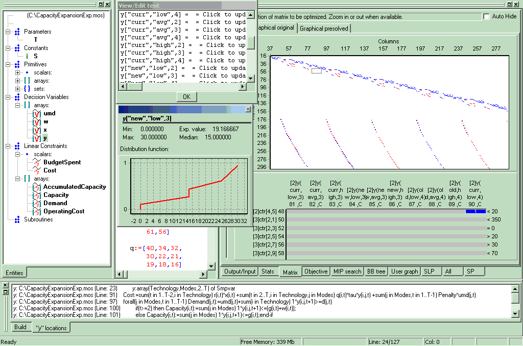
Figure 5.18: IVE SP interface
IVE provides additional features like SP scenario form, Stochastic Dashboard, and Matrix View for visualizing, manipulating, and analyzing stochastic problems.
SP scenario form
The SP form provides list, pie, and block views of the generated scenario tree.
- The list view lists the scenario indices, their probabilities, and for each stage, the realized values of sprand in that stage. Each sprand's name is prefixed by its stage number in curly brackets.
- The pie view shows the scenario tree in the form of a pie. The first stage forms the innermost circle and the last stage forms the outermost circle. Each stage is colored differently and the nodes in that stage are shaded differently. The size of the node (span of the angle in the circle) is proportional to the cumulative probability of that node (i.e., product of conditional probabilities along the branches to that node). Users can click on a node to see the path to it, its node number, its stage number, the realized values of sprand, and the conditional and cumulative probability. Users may also double-click on any node and see the realized values of each of the sprand along the path to that node. In addition, one can move the pie by clicking and holding the right mouse button and dragging. User may also zoom in and out by using the centre-wheel of the mouse.
- In the block view, the left most block corresponds to the first stage, and the last block corresponds to the last stage. Other features are similar to the ones in the pie-view features except that users can move the tree only vertically (see fig below).
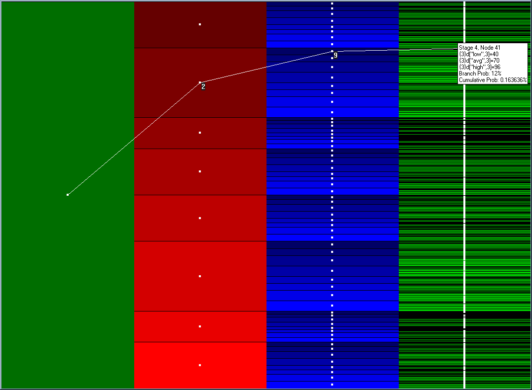
Figure 5.19: Scenario tree block view
Stochastic dashboard
The dashboard provides the model information, namely, the number of stages, spvar, sprand, splinctr, and scenarios. The dashboard also lists the sprand, spvar, splinctr, and scenario indices in the model. Each of these is prefixed by its stage number in curly brackets. The dashboard also gives a miniature version of the scenario tree in the block and the pie view. Users may click on any entity (sprand, spvar, or splinctr) to see its cumulative probability distribution (with statistics like min, max, median and expected values) across scenarios. Users may also select one or more scenarios with any entity to see its values in those scenarios (see fig below).
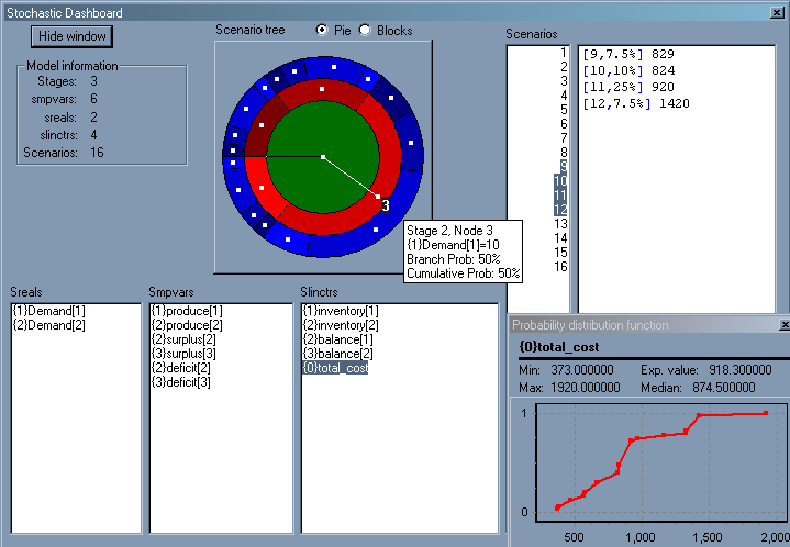
Figure 5.20: Stochastic dashboard
One may interactively aggregate and delete scenarios in IVE after scenario generation and before optimization. The user must check the option Pause to prune scenario tree manually in IVE in order to perform these scenario-pruning operations.
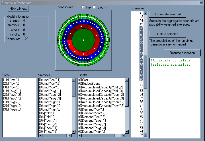
Figure 5.21: Aggregation and Deletion in IVE
Aggregation
Once the model is running in the pause mode, users may click on multiple numbers of nodes to select the scenarios to be aggregated. If the button Aggregate selected on the dashboard is pressed, then aggregation is performed automatically and the scenario tree is updated. As mentioned earlier, the new aggregated scenario probability is sum of all the probabilities of the scenarios that were aggregated, and the aggregated sprand are sum of the corresponding conditional–probability weighted sprand.
Deletion
In the pause mode, users may select scenarios to be deleted. One may use the `ctrl' key on the keyboard for multiple selections of scenarios from the scenario list or from the scenario tree, and then press the button Delete selected. The remaining scenario and conditional probabilities are re-normalized, and the scenario tree is updated automatically. Note that both of these operations can be performed interactively, and multiple times as long as a valid scenario tree exists. The equivalent mmsp functions are displayed in the text box on the dashboard, which users may copy in their model to replicate the same behavior in the next run. Users may resume execution of the model by pressing the button Resume execution on the dashboard.
Matrix View
Users may view the underlying expanded matrix in the Matrix tab in IVE. The matrix view provides List view to see the solution, and the Graphical original and Graphical presolved to visualize the original and the pre-solved matrix. The user must select the option for viewing these matrices in IVE. As mentioned in Section Expanding the underlying deterministic model, the matrix can be expanded according to nodes or scenario. In the former case, the variables and constraints are prefixed by their node numbers, whereas in the latter case they are prefixed by their scenario numbers. For the purpose of clarity, these numbers are enclosed in square brackets.
Other standard features
The following standard features of IVE can be used for writing and analyzing the stochastic models:
- Interface for modeling the problem
- Input/Output form for viewing the problem statistics and optimization log
- Branch and bound tree, if the global problem is being solved
If you have any comments or suggestions about these pages, please send mail to docs@dashoptimization.com.